Identifying and quantifying events

This notebook uses toy examples to show how to work with timewizard’s event detection functionality.

import numpy as np
import timewizard.perievent as tw
import matplotlib.pyplot as plt
from scipy.interpolate import interp1d

These functions take a one-D, binarized sigal (e.g. 0’s and 1’s), along with its timestamps, and return information about the timing of events (i.e., when the signal transitioned from 0 to 1).

Features include:

• returns a neat table with start / stop / duration statistics.

• specify a minimum block spacing; runs of 1’s interrupted by runs of 0’s which are shorter than the minimum spacing will be combined.

• easily transform a list of times into a list of “times from previous event” or “time to next event”.

Let’s return to our data from the first example, with an animal running in a circle.

np.random.seed(10)

fs = 30  # Hz
t = np.arange(0, 20*np.pi, 1/fs)  
x = np.cos(t) + np.random.random(t.shape) * 0.2
y = np.sin(t) + np.random.random(t.shape) * 0.2
data = np.hstack([x.reshape(-1,1), y.reshape(-1,1)])
plt.plot(data[:,0], data[:,1], color='gray')
_ = plt.axis('square')

Identifying events

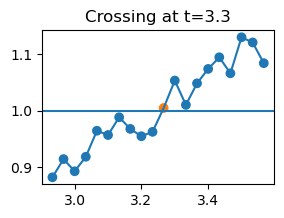
Recall that the animal preferentially vocalized around theta=pi. So, we decide to look at every instance where the animal passed theta=pi, not just the ones where it vocalized. (Perhaps we want to make some raster plots!)

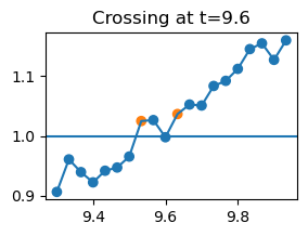
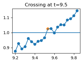
If we naively find all the moments where the animal passed theta=pi, we will end up with some very short bouts, due to the random noise in the animal’s position.

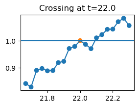
def plot_crossings():
    for i in range(len(crossing_idx)):
        s = slice(crossing_idx[i] - 10, crossing_idx[i] + 10)
        plt.figure(figsize=(3,2))
        plt.plot(t[s], theta[s]/np.pi, '-')
        plt.scatter(
            t[s], 
            theta[s]/np.pi, 
            c=['C1' if i in crossing_idx else 'C0' for i in range(s.start, s.stop)]
        )
        plt.axhline(1)
        plt.title(f'Crossing at t={t[crossing_idx[i]].round(1)}')
        if i == 3: break
    return

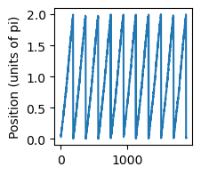
theta = np.arctan2(y, x)
theta[theta < 0] = theta[theta < 0] + 2*np.pi  # put into range (0, 2pi) for simplicity
rel_position_to_pi = np.vstack(
    [np.concatenate([[np.nan], theta[:-1] < np.pi]),
    theta > np.pi]
)  # moments where prev posn is less than pi and this one is greater
bool_train = (rel_position_to_pi.sum(axis=0) == 2)
crossing_idx = np.where(bool_train)[0]

plt.figure(figsize=(2,2))
plt.plot(theta/np.pi)
plt.ylabel('Position (units of pi)')

Text(0, 0.5, 'Position (units of pi)')

plot_crossings()  # only shows the first few, to save space

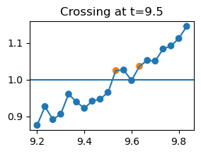
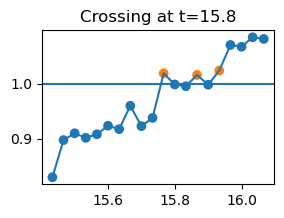
One way to get around this is to impose a minimum block length. Let’s say that if the animal crosses back within one second of an initial crossing, then we won’t count it. timewizard wraps this nicely with tw.event_times_from_train(mode='initial_onset', block_min_spacing=x)

min_spacing = 1
crossing_idx, crossing_times = tw.event_times_from_train(
    bool_train, 
    t, 
    mode='initial_onset', 
    block_min_spacing=min_spacing
)

plot_crossings()

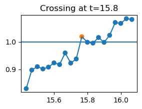
Much better!

Characterizing epochs

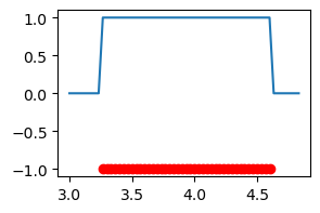
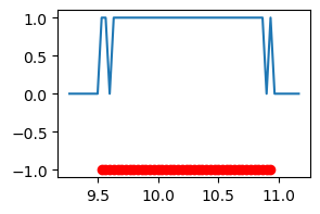
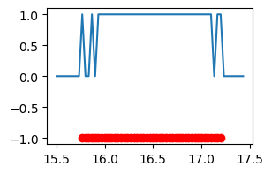
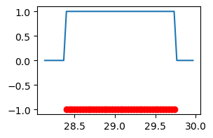
Next, a reviewer on our paper asks if we see anything during epochs when the animal is in a certain area of the arena, say the slice from np.pi to 3*np.pi/2. If we naively find onsets and offsets, we will run into the same problem as before – detecting overly short epochs due to noise. Again, timewizard wraps the desired behavior for you in tw.event_epochs.

NB: simply getting onsets + offsets with event_times_from_train will give the same results as event_epochs if there is no noise, but in noisy cases like this, event_epochs is careful to ensure the result has matched onsets + offsets, whereas you can end up with differeing numbers of onsets / offsets if you get them separately.

bool_train = (theta > np.pi) & (theta < 3*np.pi/2)
df = tw.event_epochs(bool_train, t, mode='initial_onset', block_min_spacing=min_spacing)
df

	onset_index	onset_time	offset_index	offset_time	duration	value
0	98	3.266667	139	4.633333	1.366667	1
1	286	9.533333	329	10.966667	1.433333	1
2	473	15.766667	517	17.233333	1.466667	1
3	660	22.000000	705	23.500000	1.500000	1
4	852	28.400000	893	29.766667	1.366667	1
5	1041	34.700000	1080	36.000000	1.300000	1
6	1229	40.966667	1270	42.333333	1.366667	1
7	1416	47.200000	1457	48.566667	1.366667	1
8	1605	53.500000	1648	54.933333	1.433333	1
9	1794	59.800000	1833	61.100000	1.300000	1

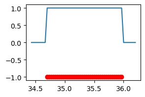
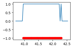
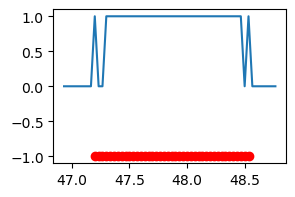
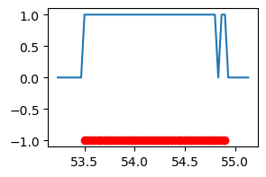
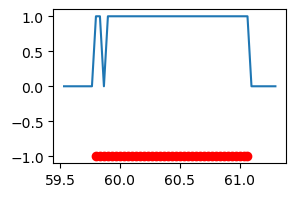
for i in range(len(df)):
    s = slice(int(df.loc[i, 'onset_index'] - fs/4), int(df.loc[i, 'offset_index'] + fs/4))
    plt.figure(figsize=(3,2))
    plt.plot(t[s], bool_train[s], '-')
    xvals = t[range(df.loc[i, 'onset_index'], df.loc[i, 'offset_index'])]
    plt.scatter(xvals ,np.repeat(-1, len(xvals)), c='r')